Coordinate Systems and Transformations
This package defines common coordinate systems used in heliophysics and space physics research.
Standard Coordinate Systems
Systems based on the Earth-Sun line
- GSE (Geocentric Solar Ecliptic)
- GSM (Geocentric Solar Magnetic)
Systems based on the Earth's rotation axis
- GEO (Geographic)
- GEI (Geocentric Equatorial Inertial)
- J2000
Systems based on the dipole axis of the Earth's magnetic field
- SM (Solar Magnetic)
- MAG (Geomagnetic)
Other coordinate systems
More information can be found in the the following links
Coordinate Transformations
SPEDAS.rotate — Function
rotate(da, mats)Rotate a dimensioned array using a vector of rotation matrices aligned to its time axis. Requires DimensionalData to be loaded.
A comprehensive description of the transformations can be found in Hapgood [1]
Coordinate transformations between geocentric systems
SPEDAS.cotrans — Function
cotrans(out, A, [times]; in=get_coord(A), backend=GeoCotrans)
cotrans(in => out, A, [times]; backend=GeoCotrans)
Transform data to the out coordinate system.
By default, this uses Julia's GeoCotrans. Use backend = IRBEM after loading IRBEM.jl to call Fortran's IRBEM implementation.
References:
- IRBEM-LIB: compute magnetic coordinates and perform coordinate conversions (Documentation, IRBEM.jl)
- SPEDAS Cotrans
using DimensionalData
using Speasy, SPEDAS
using CairoMakie, SpacePhysicsMakie

pos_gse = get_data("cda/THC_L1_STATE/thc_pos_gse", "2015-10-16", "2015-10-17") |> DimArray

pos_gsm = cotrans(:GSM, pos_gse)
pos_sm = cotrans(:SM, pos_gsm)
pos_geo = cotrans(:GEO, pos_gsm)

tplot((pos_gse, pos_gsm, pos_sm, pos_geo))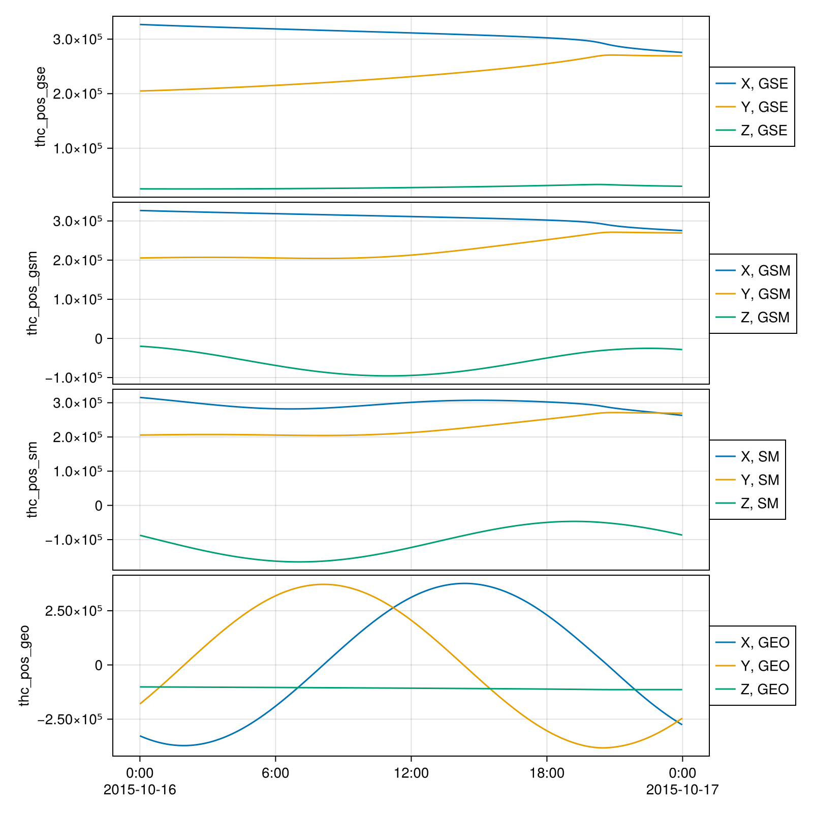
Specialized Coordinate Systems
The package also provides transformations for analysis-specific coordinate systems:
Field-Aligned Coordinates (FAC)
A local coordinate system defined relative to the ambient magnetic field direction, useful for studying plasma waves and particle distributions.
SPEDAS.fac_mat — Function
fac_mat(vec::AbstractVector; xref=[1.0, 0.0, 0.0])Generates a field-aligned coordinate (FAC) transformation matrix for a vector.
Arguments
vec: A 3-element vector representing the magnetic field
Minimum Variance Analysis (MVA) and Boundary Normal Coordinates (LMN)
A coordinate system derived from the eigenvalues and eigenvectors of the magnetic field variance matrix, commonly used in analyzing current sheets, discontinuities, and wave propagation.
See MinimumVarianceAnalysis.jl for more details.
MinimumVarianceAnalysis.mva_eigen — Function
mva_eigen(x::AbstractMatrix; dim = nothing, sort=(;), check=false) -> F::EigenPerform minimum variance analysis of the magnetic field B or maximum variance analysis of the electric field E when field=:E.
x varies along the dim dimension.
Return Eigen factorization object F which contains the eigenvalues in F.values and the eigenvectors in the columns of the matrix F.vectors. The kth eigenvector can be obtained from the slice F.vectors[:, k].
Set check=true to check the reliability of the result.
Notes
For a one-dimensional current layer, the tangential electric field components are approximately constant across the boundary, while the normal component exhibits the largest variation. Therefore, the eigenvector corresponding to the maximum eigenvalue $λ_1$ (first column of F.vectors) gives an estimate of the boundary normal direction.
MinimumVarianceAnalysis.mva — Function
mva(V, F=V; dim=nothing, kwargs...)Transform a timeseries V into the LMN coordinate system based on the minimum/maximum variance analysis of reference field F along the dim dimension (time).
MinimumVarianceAnalysis.check_mva_eigen — Function
check_mva_eigen(F; r0=5, verbose=false, field = :B)Check the quality of the MVA result.
If λ₁ ≥ λ₂ ≥ λ₃ are 3 eigenvalues of the constructed matrix M. For MVAB, a good indicator of nice results should have $|λ₂ / λ₃| > r₀$ (default $r₀ = 5$).
For MVAE, a reliable normal direction requires the maximum eigenvalue $λ₁$ to be well-separated from the intermediate eigenvalue $λ₂$. The ratio $|λ₁ / λ₂| > r₀$ is used as a quality indicator.
See also: Comparison with PySPEDAS.
Reference
- PySPEDAS: Coordinate Systems
- geopack: Python version of geopack and Tsyganenko models
- geospacelab: A python-based library to collect, manage, and visualize geospace data (e.g. OMNI, geomagnetic indices, EISCAT, DMSP, SWARM, TEC, AMPERE, etc.).
- aacgmv2: Python library for AACGM-v2 magnetic coordinates