Examples
Computing
Working with Units
By default, positions are in planetary radii
using PlanetaryMagneticFields
using Unitful
model = JRM09()
r_km = 107238.0u"km"  # 1.5 RJ in km
θ, φ = π/4, 0.0
@assert model(r_km, θ, φ) == model(1.5, θ, φ)
model(r_km, θ, φ)
3-element StaticArraysCore.SVector{3, Float64} with indices SOneTo(3):
117871.89135977793
92648.1424209409
-12029.869015050079Computing on multiple positions
using PlanetaryMagneticFields

model = JRM09()

# Evaluate at different positions
positions = [
    (1.5, 0.0, 0.0),      # North pole, 1.5 RJ
    (2.0, π/2, 0.0),      # Equator, 2 RJ
    (1.0, π/4, π/2),      # 45° colatitude, 90° longitude
]
B = model.(positions)
3-element Vector{StaticArraysCore.SVector{3, Float64}}:
[227836.64536639338, -0.00738649790722077, 0.0]
[-9573.896513591537, 45457.37988446424, -3151.0162735670015]
[286982.526589615, 529841.9205580986, 38158.69343083006]Computing on a Grid
You can compute field values over a latitude-longitude grid:
# Compute field vectors at 1.5 planetary radii
r = 1.5
field = fieldmap(model, r; nlat=90, nlon=180)
Br = getindex.(field, 1)
# Field statistics
println("Br range: $(minimum(Br)) to $(maximum(Br)) nT")
Br range: -253611.79461533582 to 314494.24951135577 nTUsing Cartesian Coordinates
# Cartesian input and output
model = JRM09()
x, y, z = 1.0, 0.5, 0.5  # In Jupiter radii
B = model(x, y, z; from=:cartesian) # by default, output format follows input format

# Cartesian input, spherical output
model(x, y, z; from=:cartesian, to=:spherical)
3-element StaticArraysCore.SVector{3, Float64} with indices SOneTo(3):
107520.10842292434
182556.05651367328
-22200.53686085128Visualization
using CairoMakie, GeoMakie
using PlanetaryMagneticFields
Different Projections
Various map projections are supported via PROJ strings:
model = load_model(:earth, "igrf2020")

let fig = Figure(size=(1200, 400))
    sf1 = plot_fieldmap(fig[1, 1], model; axis=(; title="Mollweide"), dest="+proj=moll")
    sf2 = plot_fieldmap(fig[1, 2], model; axis=(; title="Robinson"), dest="+proj=robin")
    sf3 = plot_fieldmap(fig[1, 3], model; axis=(; title="Equal Earth"), dest="+proj=eqearth")
fig
end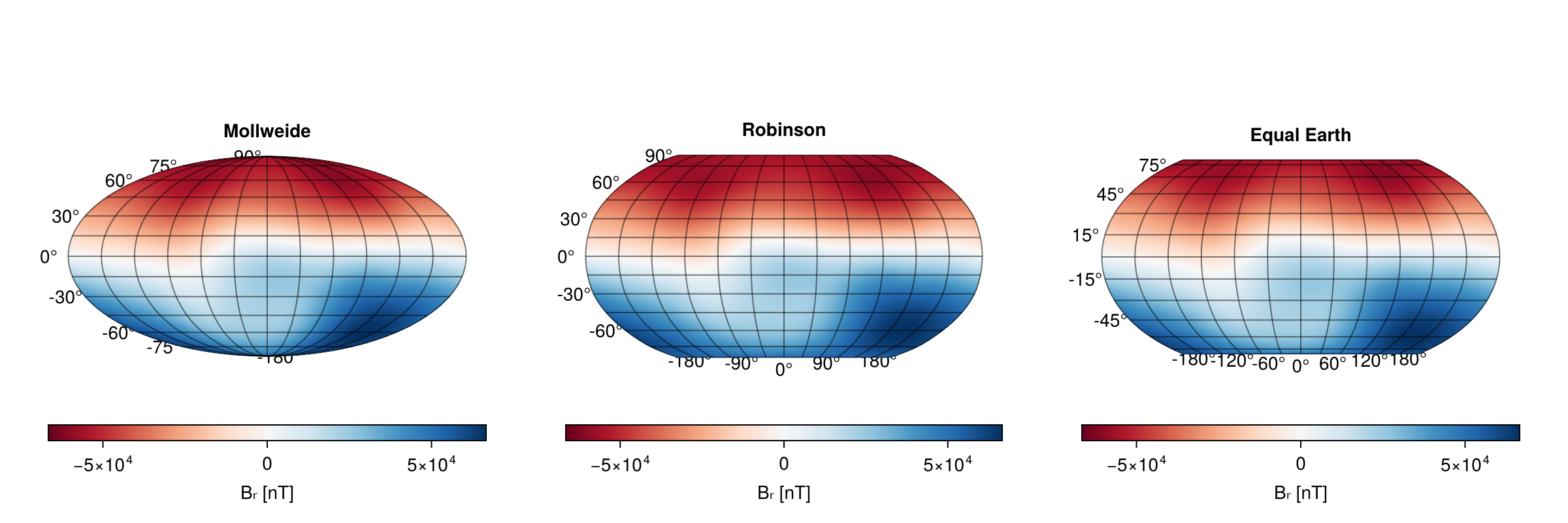
Plotting All Planets
Create a comprehensive figure showing magnetic field maps for all supported planets:
plot_models(; r=0.9, figure = (; size=(1200, 400)), position = Makie.Right())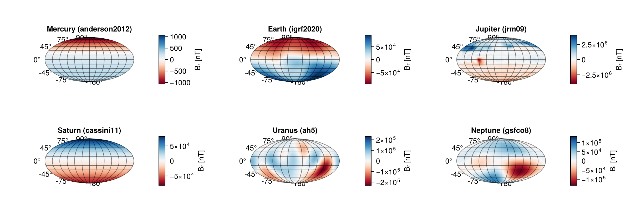
This displays the radial magnetic field (Bᵣ) at the surface for:
- Mercury (Anderson 2012 model)
- Earth (IGRF 2020 model)
- Mars (Langlais 2019 crustal field model)
- Jupiter (JRM09 model)
- Saturn (Cassini 11 model)
- Uranus (AH5 model)
- Neptune (GSFC O8 model)
- Ganymede (Kivelson 2002 model)
Custom Multi-Planet Figures
You can create custom layouts with specific planets and models:
# Giant planets comparison
planets = [
    (:Jupiter, "JRM09"),
    (:Saturn, "Cassini11"),
    (:Uranus, "AH5"),
    (:Neptune, "GSFCO8"),
]
models = map(planets) do (planet, model_name)
    load_model(planet, model_name)
end
4-element Vector{PlanetaryMagneticFields.SphericalHarmonicModel{PlanetaryMagneticFields.GaussCoefficients{Matrix{Float64}}, PlanetaryMagneticFields.Planet, PlanetaryMagneticFields.PlanetFrame}}:
SphericalHarmonicModel(name=JRM09, obj=PlanetaryMagneticFields.Planet(:jupiter, 71492.0), degree=20, order=20)
SphericalHarmonicModel(name=Cassini11, obj=PlanetaryMagneticFields.Planet(:saturn, 60268.0), degree=12, order=0)
SphericalHarmonicModel(name=AH5, obj=PlanetaryMagneticFields.Planet(:uranus, 25559.0), degree=4, order=4)
SphericalHarmonicModel(name=GSFCO8, obj=PlanetaryMagneticFields.Planet(:neptune, 24764.0), degree=3, order=3)plot_models(; r=0.9, models = models[1:2])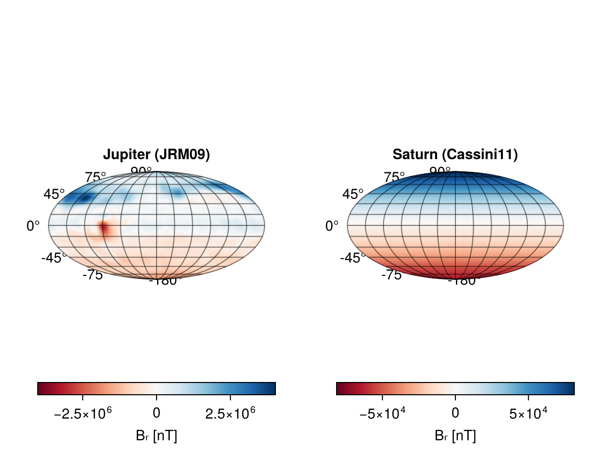
let fig = Figure()
    fpos = [(1, 1), (1, 2), (2, 1), (2,2)]
    for (idx, (planet, model_name)) in enumerate(planets)
        ax = GeoAxis(fig[fpos[idx]...];  title="$(planet) => $(model_name)")
        sf = plot_fieldmap!(ax, models[idx]; r=1.0)
    end
    Label(fig[0, :], "Giant Planet Magnetic Fields")
    fig
end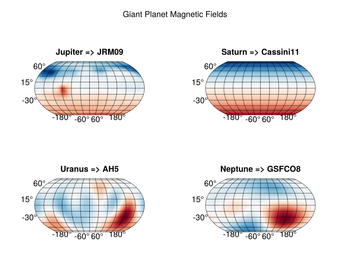
Tracing Field Lines (Jupiter)
trace from GeoCotrans integrates du/ds = ±B̂(u) along arc length.
This reproduces the JRM33 panel of JupiterMag's PlotRhoZ example: 8 field lines starting on the surface in the noon meridian (φ=0), traced both directions to give closed footpoint-to-footpoint loops, then projected into the ρ–z plane where ρ = √(x² + y²).
using OrdinaryDiffEqTsit5                     # any SciML solver works
using PlanetaryMagneticFields: PlanetFrame    # for the Cartesian-input frame

model = JRM33()

n = 8
# Surface starts at φ = 0, southern-hemisphere colatitudes 145°…157.5°
colats = deg2rad.(180 .- range(22.5, 35, length = n))
starts = [[sin(θ), 0.0, cos(θ)] for θ in colats]

options = (; from = (PlanetFrame(), Cartesian3()), r0 = 0.95, rlim = 20.0, maxs = 80.0, dtmax = 0.05)

lines = map(starts) do pos
    fwd = trace(pos, nothing, Tsit5(); model, dir =  1, options...)
    bwd = trace(pos, nothing, Tsit5(); model, dir = -1, options...)
    vcat(reverse(bwd.u), fwd.u)
end

fig = Figure(size = (650, 400))
ax = Axis(fig[1, 1]; aspect = DataAspect(), xlabel = "ρ [RJ]", ylabel = "z [RJ]",
          title = "Jupiter (JRM33) field lines")
poly!(ax, Circle(Point2f(0, 0), 1.0f0); color = (:tan, 0.4), strokecolor = :tan)
for line in lines
    lines!(ax, [hypot(u[1], u[2]) for u in line], [u[3] for u in line];
           color = :black, linewidth = 1.2)
end
xlims!(ax, -2, 15); ylims!(ax, -6, 6)
fig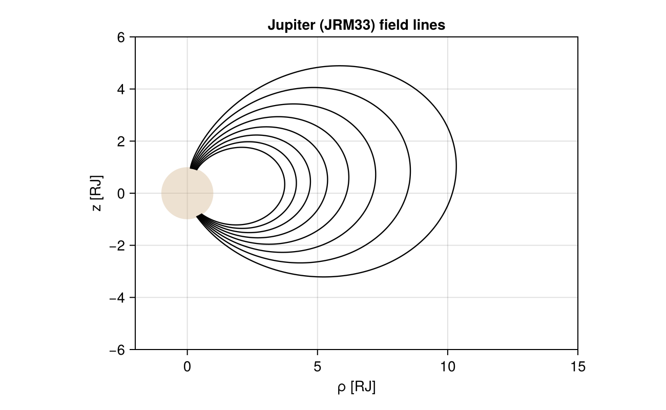
trace keywords used above:
dir = ±1— parallel / anti-parallel to Br0,rlim— inner / outer termination radii in planetary radiimaxs— maximum arc length (cuts off lines that wander)
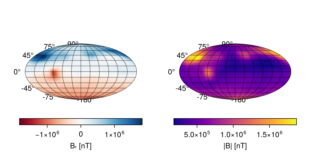
Different Field Components
Plot different components of the magnetic field:
using LinearAlgebra: norm

model = load_model(:jupiter, "jrm09")
let fig = Figure(; size=(600, 300))
    # Radial component
    plot_fieldmap(fig[1, 1], model; idx=1)
    # Field magnitude
    plot_fieldmap(fig[1, 2], model; idx=norm, colormap=:plasma)
    fig
end