Field Line Tracing

Basic Usage

using GeoCotrans, OrdinaryDiffEqTsit5, Dates

# Define time for field evaluation
t = DateTime(2020, 1, 1)

# Trace a field line starting from [3, 0, 0] Earth radii (GEO coordinates)
sol = trace(GEO(3.0, 0.0, 0.0), t, Tsit5())

retcode: Terminated
Interpolation: specialized 4th order "free" interpolation
t: 12-element Vector{Float64}:
 0.0
 0.0009999885482375654
 0.028570064912686398
 0.1407684080982351
 0.3519749672311441
 0.6431698683965004
 1.024306661606543
 1.5081972108001358
 2.099085981289496
 2.792534178589731
 3.205956676634449
 3.205956676634449
u: 12-element Vector{StaticArraysCore.SVector{3, Float64}}:
 [3.0, 0.0, 0.0]
 [3.000024874434897, -0.00014500231793512512, 0.0009891069741289906]
 [3.0003235012472826, -0.004134458625726653, 0.02826652634920791]
 [2.993848453320644, -0.02015350777736001, 0.1390692215146891]
 [2.9488860092075475, -0.048843247209553714, 0.3430541747614227]
 [2.8224968633836514, -0.08360127134311553, 0.602120044818346]
 [2.5662811017774287, -0.11798135726090243, 0.8800721963429805]
 [2.1440347161854936, -0.1414701133669414, 1.110356322822682]
 [1.563090620582933, -0.14097171618276977, 1.1992211601268272]
 [0.8913228125031449, -0.1060612201590972, 1.0500477268481536]
 [0.5381592102106133, -0.07300633778734437, 0.8396753772192972]
 [0.5381592102106133, -0.07300633778734437, 0.8396753772192972]

Plotting with Makie

Here's a complete example showing how to trace and visualize magnetic field lines using GLMakie:

using GeoCotrans, OrdinaryDiffEqTsit5, Dates
using CairoMakie

# Time for field evaluation
t = DateTime(2020, 1, 1)

# Create figure
fig = Figure(size = (800, 800))
ax = Axis3(fig[1, 1],
    xlabel = "X (Re)",
    ylabel = "Y (Re)",
    zlabel = "Z (Re)",
    title = "IGRF Field Lines at $(Date(t))",
    aspect = :data
)

# Draw Earth (unit sphere)
θ_sphere = range(0, π, length=30)
φ_sphere = range(0, 2π, length=60)
x_sphere = [sin(θ) * cos(φ) for θ in θ_sphere, φ in φ_sphere]
y_sphere = [sin(θ) * sin(φ) for θ in θ_sphere, φ in φ_sphere]
z_sphere = [cos(θ) for θ in θ_sphere, φ in φ_sphere]
surface!(ax, x_sphere, y_sphere, z_sphere, color = :lightblue, alpha = 0.8)

# Trace field lines from different starting positions
L_values = [2.0, 3.0, 4.0, 5.0]  # L-shell values
colors = [:red, :orange, :green, :blue]

for (L, color) in zip(L_values, colors)
    # Trace in both directions from the equator
    for dir in [1, -1]
        sol = trace(GEO(L, 0.0, 0.0), t, Tsit5(); dir = dir)
        # Plot the field line
        plot!(ax, sol; color = color, linewidth = 2, idxs = (1, 2, 3),
            label = dir == 1 ? "L = $L" : nothing)
    end
end

axislegend(ax, position = :rt) # Add legend
limits!(ax, -6, 6, -6, 6, -6, 6) # Set view limits

fig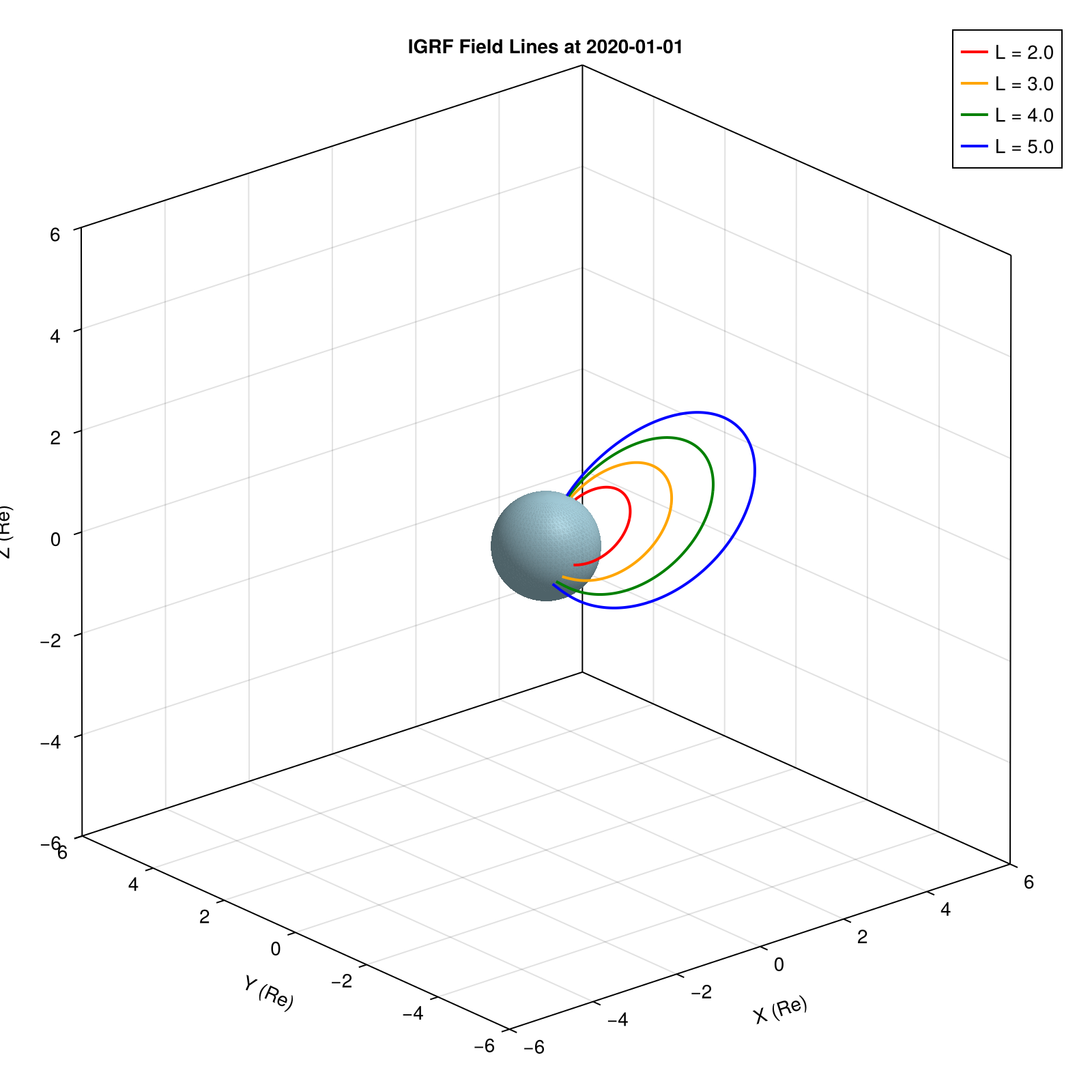

2D Visualization

using GeoCotrans, OrdinaryDiffEqTsit5, Dates
using CairoMakie

t = DateTime(2020, 1, 1)

fig = Figure(size = (1000, 500))

# Left panel: Meridional plane (X-Z)
ax1 = Axis(fig[1, 1],
    xlabel = "X (Re)", ylabel = "Z (Re)",
    title = "Field Lines in Meridional Plane",
    aspect = DataAspect()
)

# Draw Earth cross-section
θ_circle = range(0, 2π, length=100)
lines!(ax1, cos.(θ_circle), sin.(θ_circle), color = :lightblue, linewidth = 3)

# Trace field lines
for L in [2.0, 3.0, 4.0, 5.0, 6.0]
    for dir in [1, -1]
        sol = trace(GEO(L, 0.0, 0.0), t, Tsit5(); dir = dir)
        lines!(ax1, sol, idxs = (1, 3), color = :darkblue, linewidth = 1.5)
    end
end

limits!(ax1, -7, 7, -7, 7)

# Right panel: Equatorial plane (X-Y)
ax2 = Axis(fig[1, 2],
    xlabel = "X (Re)", ylabel = "Y (Re)",
    title = "Field Lines in Equatorial Plane",
    aspect = DataAspect()
)

# Draw Earth cross-section
lines!(ax2, cos.(θ_circle), sin.(θ_circle), color = :lightblue, linewidth = 3)

# Starting points slightly off equator to see field line structure
for L in [3.0, 4.0, 5.0]
    for φ in range(0, 2π, length=13)[1:12]
        y0, x0 = L .* sincos(φ)
        # Start slightly above equator
        sol = trace(GEO(x0, y0, 0.1), t, Tsit5(); dir = 1)
        lines!(ax2, sol, idxs = (1, 2), color = :darkgreen, linewidth = 1)
    end
end

limits!(ax2, -7, 7, -7, 7)

fig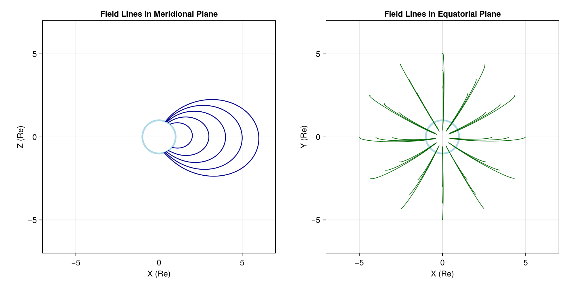

API Reference

FieldLineProblem(pos, tspan, t; model=IGRF(), dir=1)

using GeoCotrans, OrdinaryDiffEqTsit5, Dates

t = DateTime(2020, 1, 1)
pos = [3.0, 0.0, 0.0]
prob = FieldLineProblem(pos, (0.0, 50.0), t)
sol = solve(prob, Tsit5())

FieldLineCallback(; r0=1.0, rlim=10.0)

trace(pos, t, solver; kwargs...) :: ODESolution

using GeoCotrans, OrdinaryDiffEqTsit5
sol = trace([3.0, 0.0, 0.0], t, Tsit5())